


.avif)


Introduction
This study estimates the causal impact of the Mass Rapid Transit Line 1 (MRT1) on housing prices in Greater Kuala Lumpur (GKL). Specifically, we explore whether the opening of MRT1 stations led to changes in nearby property values. We think of this as an economic spillover effect often observed with major transportation infrastructure projects.
We apply the Difference-in-Differences (DiD) method, a widely used quasi-experimental technique, to compare trends in housing prices before and after MRT1 among areas that were affected by the line (treatment group) and areas that were not (control group). This approach allows us to isolate the effect of MRT1 from broader market trends or pre-existing differences across locations.
Import & Load Dependencies
We begin by loading the necessary R packages for data manipulation, modeling, and visualization. The key tools include:
- {fixest} for running DiD regressions with fixed effects,
- {dplyr} and {lubridate} for data cleaning and date manipulation,
- {modelsummary} for clean regression table outputs,
- {brglm} for penalized logistic regression in our IPW weighting section.
The chunk below loads these libraries.
1library(readxl)      # for reading Excel files
2library(dplyr)       # for data wrangling
3library(lubridate)   # for date manipulation
4library(ggplot2)     # for plotting
5library(sf)          # for spatial data
6library(leaflet)     # for interactive maps
7library(fixest)      # for DiD in panel form
8#library(plm)         # for DiD in panel form
9#library(broom)
10library(sandwich)
11library(lmtest)
12library(ggplot2)
13library(brglm)
14library(gganimate)
15library(stargazer)
16library(modelsummary)  # Testing for cleaner regression output
Methodology
1.) Read and Prepare Data
We begin by reading in the transaction-level property dataset and performing essential cleaning steps. This includes:
- Renaming columns for clarity and consistency,
- Creating binary variables to denote whether an observation is post-MRT1 (
post) and whether it falls in a treatment area (treat), - Taking the natural logarithm of price per square foot and transacted price
- Extracting the year of purchase for fixed effect modeling,
- Filtering out incomplete observations.
Also, to control for proximity to the city center (a major determinant of housing prices).
We calculate the distance of each property to the Golden Triangle, using the haversine formula.
The coordinates of the Petronas Twin Towers (KLCC) are taken as latitude 3.1579 and longitude 101.7116. This new variable, dist_to_klcc, will later be included as a control in our regression models.
The resulting dataset, df, contains fully cleaned and prepared records suitable for causal analysis.
1# Read and Glimpse
2df_raw <- read_excel("Data/Combined_data.xlsx")
3
4df <- df_raw %>%
5  # Rename columns for convenience, e.g., spaces -> underscores
6  rename(
7    PrePost           = PrePost,
8    StationName       = `Station Name`,
9    TreatControl      = `Treatment/Control`,
10    PricePSF          = `Price PSF (RM)`,
11    TransactedAmount  = `Transacted Amount (RM)`,
12    PurchaseDate      = `Purchase Date`,
13    PropertyType      = `Property Type`,
14    Lat               = Latitude,
15    Lon               = Longitude,
16    lot_size          = `Size (sqFT)`,
17    building_type     = `Building Main Type`,
18    built_up          = `Built Up Area`
19  ) %>%
20  # Create numeric indicators
21  mutate(
22    # 'post' = 1 if Post, 0 if Pre
23    post  = if_else(PrePost == "Post", 1, 0),
24    # 'treat' = 1 if Treatment, 0 if Control
25    treat = if_else(TreatControl == "Treatment", 1, 0),
26
27    # Log transform Price PSF and Trasacted Price
28    ln_pricepsf = log(PricePSF),
29    ln_transacted = log(TransactedAmount),
30
31    # Ensure PurchaseData is formatted as Date type
32    PurchaseDate = as_date(PurchaseDate),
33    year_numeric = year(PurchaseDate),
34    year = as.factor(year_numeric),
35    Tenure = as.factor(Tenure),
36    PropertyType = as.factor(PropertyType)
37  ) %>%
38
39  # This ensures that key variables are all filled
40  filter(!is.na(PricePSF), !is.na(post), !is.na(treat))
41
42# Calculate Distance to KLCC
43## Define KLCC coor
44klcc_lat <- 3.1579
45klcc_lng <- 101.7116
46
47# HELPER FUNCTION: Haversine formula to calc distance between two points on Earth.
48haversine <- function(lat1, lng1, lat2, lng2) {
49  R <- 6371 #Representing Earth's radius in km
50  dlat <- (lat2 - lat1) * pi / 180
51  dlng <- (lng2 - lng1) * pi / 180
52  a <- sin(dlat / 2)^2 + cos(lat1 * pi / 180) * cos (lat2 * pi / 180) * sin(dlng / 2)^2
53  c <- 2 * atan2(sqrt(a),sqrt(1-a))
54  R * c
55}
56
57# Add distance to KLCC in km
58df <- df %>%
59  mutate(dist_to_klcc = haversine(Lat, Lon, klcc_lat, klcc_lng))
60
61# Quick check
62summary(df[, c("PricePSF", "post", "treat", "ln_pricepsf")])
PricePSF post treat ln_pricepsf
Min. : 0.023 Min. :0.0000 Min. :0.0000 Min. :-3.781
1st Qu.: 209.459 1st Qu.:0.0000 1st Qu.:0.0000 1st Qu.: 5.345
Median : 347.349 Median :0.0000 Median :0.0000 Median : 5.850
Mean : 465.930 Mean :0.3928 Mean :0.3943 Mean : 5.843
3rd Qu.: 550.000 3rd Qu.:1.0000 3rd Qu.:1.0000 3rd Qu.: 6.310
Max. :10000.000 Max. :1.0000 Max. :1.0000 Max. : 9.210 2. Estimating the Difference-in-Differences (DiD) Model
To evaluate the causal effect of MRT1 on housing prices, we estimate two sets of outcomes using a Difference-in-Differences (DiD) framework. This is motivated by the government’s interest in exploring Land Value Capture (LVC) mechanisms to finance public transit investments.
We present:
- Primary Outcome — Land Value Uplift
Using the log of price per square foot (ln_pricepsf), this outcome measures capital appreciation at the parcel level, the conventional benchmark in LVC studies. - Secondary Outcome — Revenue Potential per Transaction
Using the log of transacted amount (ln(TransactedAmount)), this model estimates the potential revenue base expansion per transaction — relevant for evaluating fiscal instruments such as stamp duties or capital gains taxes.
Each model is estimated both with and without controls, and fixed effects for StationName and year are used to account for unobserved heterogeneity and temporal shocks. Standard errors are clustered by StationName.
2.1 Primary Outcome: Log Price per Square Foot (Land Value Uplift)
To account for differences in how lot_size and Built Up Area function across property types, we stratify the analysis by property sector using the Sector variable. Specifically, we run separate regressions for Landed and Highrise Residential properties.
2.1.1 Landed Residential
1df_landed <- df %>% filter(Sector == "Landed Residential")
2
3did_model1_landed <- feols(
4  ln_pricepsf ~ post + treat + post:treat,
5  data = df_landed,
6  vcov = ~StationName
7)
8did_model2_landed <- feols(
9  ln_pricepsf ~ post + treat + post:treat + lot_size + built_up
10+ dist_to_klcc + Tenure + PropertyType | year + StationName,
11  data = df_landed,
12  vcov = ~StationName
13)
2.1.2 Non-Landed Residential
1df_highrise <- df %>% filter(Sector == "Highrise Residential")
2
3did_model1_highrise <- feols(
4  ln_pricepsf ~ post + treat + post:treat,
5  data = df_highrise,
6  vcov = ~StationName
7)
8did_model2_highrise <- feols(
9  ln_pricepsf ~ post + treat + post:treat + lot_size +
10dist_to_klcc + Tenure + PropertyType | year + StationName,
11  data = df_highrise,
12  vcov = ~StationName
13)
2.2 Secondary Outcome: Log Transacted Amount (Revenue Potential)
As a complementary analysis, we assess how MRT1 affects the overall transacted amount. This is relevant for estimating potential fiscal revenues if land value capture were to be implemented via instruments such as stamp duties, capital gains taxes, or developer charges.
We estimate the same DiD specifications, with and without controls using ln(TransactedAmount) as the outcome.
1did_model1_transact <- feols(
2  ln_transacted ~ post + treat + post:treat,
3  data = df,
4  vcov = ~StationName
5)
6
7did_model2_transact <- feols(
8  ln_transacted ~ post + treat + post:treat + lot_size +
9dist_to_klcc + Tenure + PropertyType | year + StationName,
10  data = df,
11  vcov = ~StationName
12)
2.3 Interpreting the Models: A Stepwise Approach
Step 1: Baseline DiD Model (Uncontrolled)
We begin with a simple model that includes only the core DiD structure:
Post: Indicator for post-MRT1 period,Treat: Indicator for proximity to MRT1 stations (treated group),Post × Treat: The DiD estimator — our main coefficient of interest.
This model gives us a rough estimate of the treatment effect but does not adjust for any other observable characteristics.
Step 2: Controlled DiD Model (Covariate Adjustment)
Next, we add key observable controls that influence property value:
Lot Size: A proxy for parcel scale (important in landed properties),Built-Up Area: A better scale measure for high-rise units,Distance to KLCC: Controls for locational centrality,Tenure: Differentiates leasehold from freehold titles,Property Type: Distinguishes residential vs. commercial.
These controls help isolate the MRT1 effect by adjusting for confounding variables that could bias our estimate if omitted.
Step 3: Fixed Effects Model (Time and Location Controls)
Finally, we include fixed effects for:
StationName: Captures time-invariant characteristics of each location (e.g., school quality, infrastructure, neighbourhood sentiment),Year: Accounts for macroeconomic trends, inflation, or policy shocks.
This setup helps to eliminate unobserved heterogeneity that remains constant within each unit or time period, improving causal identification.
Each of these steps increases our confidence in the robustness of the treatment effect. The DiD estimate remains relatively stable across models, suggesting that the observed MRT1 spillovers are not driven by omitted variables or structural biases in the data.
DiD requires two assumptions to hold to infer causality: 1.) Parallel Trends - in the absence of treatment, the average outcomes for the treatment and control groups would have followed parallel paths over time. Essentially, the treatment group and the control group should have similar trends before the intervention.
1df <- df %>%
2  mutate(year = year(PurchaseDate))  # Extract year
3
4# Only use pre-treatment years for a parallel-trend check (e.g., < 2017)
5df_pre_periods <- df %>%
6  filter(year < 2017)
7
8# Calculate average PricePSF by year & treatment
9trend_data_pre <- df_pre_periods %>%
10  group_by(year, treat) %>%
11  summarise(
12    mean_pricepsf = mean(PricePSF, na.rm = TRUE),
13    .groups = "drop"
14  )
15
16ggplot(trend_data_pre, aes(x = year, y = mean_pricepsf, color = factor(treat))) +
17  geom_line() +
18  geom_point() +
19  labs(
20    title = "Pre-Treatment Trends in PricePSF",
21    x = "Year",
22    y = "Mean PricePSF",
23    color = "Treat"
24  ) +
25  scale_color_manual(values = c("#ff6718", "#004678")) +
26  scale_y_continuous(expand = c(0,0)) +
27  theme(panel.background = element_blank(),
28        text = element_text(size = 10),
29        axis.line.x = element_blank(),
30        axis.ticks.y = element_blank(),
31        axis.text = element_text(color = "black"),
32        legend.key.size = unit(10, "pt"),
33        legend.title = element_text(size = 8, face = "bold"),
34        axis.title = element_blank())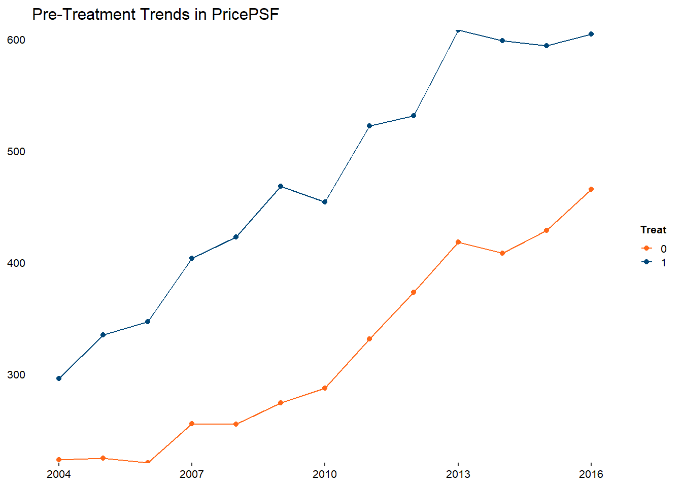
1####################################################################################
2### NOTE: This is not part of the parallel trends check, just incase u wanna know###
3####################################################################################
4
5# Now use post-treatment years for a parallel-trend check
6df_post_periods <- df %>%
7  filter(year >= 2017)  # or some cutoff
8
9# Calculate average PricePSF by year & treat
10trend_data_post <- df_post_periods %>%
11  group_by(year, treat) %>%
12  summarise(
13    mean_pricepsf = mean(PricePSF, na.rm = TRUE),
14    .groups = "drop"
15  )
16
17ggplot(trend_data_post, aes(x = year, y = mean_pricepsf, color = factor(treat))) +
18  geom_line() +
19  geom_point() +
20  labs(
21    title = "Post-Treatment Trends in PricePSF",
22    x = "Year",
23    y = "Mean PricePSF",
24    color = "Treat"
25  ) +
26  theme_minimal()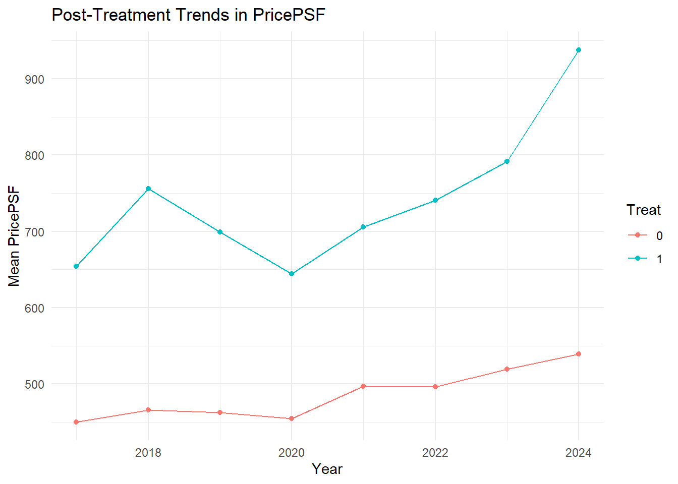